Getting started with the metapopbio package

# devtools::install_github("AldridgeCaleb/meta-pop-bio")
library(metapopbio)
#> Loading required package: openxlsx
#> Loading required package: zeallot

About

The metapopbio package is inspired by and complements the functionalities of the popbio package. Users can construct and analyze projection matrix models for metapopulations classified by age or stage and located in distinct patches.

The functionality to date is largely based on Hunter and Caswell (2005) to construct and analyze spatial matrix population models using the vec-permutation matrix. This model extends the Leslie matrix (Leslie 1945) to include dispersal rates between patches. An analogous approach was taken by Lebreton (1996) and called the “renewal equation approach.”

Current plans include support for classic metapopulation models of Gotelli (1991; 2008) and others, i.e., $\frac{df}{dt}=p_{i}(1-f)-p_{e}f$ , $\frac{df}{dt}=p_{i}(1-f)-ef(1-f)$ , $\frac{df}{dt}=if(1-f)-p_{e}f$ , and $\frac{df}{dt}=if(1-f)-ef(1-f)$ , and hyperstate matrix models (Roth and Caswell 2016). Additionally, Hanski’s (1994) incidence function $J_{i}=\frac{1}{1+\Bigl(1+\bigl[\frac{y'}{S_{i}}\bigr]^2\Bigr)\frac{e}{A_{i}^x}}$ and a metapopulation version of the Susceptible–Infected–Recovered model (SIR model), also referred to as a patch model, are also being considered. Other suggestions can be submitted in email to caleb.a.aldridge@gmail.com or as an issue on the package’s GitHub repository (https://github.com/AldridgeCaleb/meta-pop-bio/issues).

Examples

The following two examples come from Hunter and Caswell (2005) using peregrine falcon (Falco peregrinus) data from Wootton and Bell (1992) and black-headed gull (Larus ridibundus) data from Lebreton (1996).

The peregrine falcon

1. Patches, stages, and grouping

First, we define the number of patches (discrete locations) and stages (age, class, or size). In this example there are two “patches”, Northern California and Southern California, and two life-stages, juvenile and adult. We also group or will project stages within patches¹.

n_patches <- 2
n_stages <- 2
group_by <- "patches"

2. Construct vec-permutation matrix

Next, we construct the vec-permutation matrix. Essentially, the vec-permutation matrix helps us relate demographic and dispersal parameters so that populations in patches are projected considering births, immigration, deaths, and emigration (BIDE) or recruitment, immigration, survival, and emigration (RISE). The metapopbio::vec.perm function helps us to easily construct a vec-permutation matrix.

(P <-
  metapopbio::vec.perm(n_stages = n_stages,
           n_patches = n_patches,
           group_by = group_by))
#>      [,1] [,2] [,3] [,4]
#> [1,]    1    0    0    0
#> [2,]    0    0    1    0
#> [3,]    0    1    0    0
#> [4,]    0    0    0    1

3. Demographic parameters for each patch

We now specify transition probabilities from one stage to the next (survival s and recruitment r). Numbers in object names indicate patch then stage. Only adults are assumed to reproduce.

Northern first.

# Northern
f11 <- 0.00 
f12 <- 0.26
s11 <- 0.72
s12 <- 0.77

Now Southern.

# Southern
f21 <- 0.00
f22 <- 0.19  
s21 <- 0.72
s22 <- 0.77

4a. Structure demographic parameters

Now we will construct demographic (Leslise-style) matrices for each of the patches. This is just placing the demographic parameters from above into an ordered matrices for analysis and projecting.

# Northern
(B1x <-
  matrix(c(f11, f12, s11, s12),
         nrow = n_stages,
         ncol = n_stages,
         byrow = TRUE))
#>      [,1] [,2]
#> [1,] 0.00 0.26
#> [2,] 0.72 0.77
# Southern
(B2x <-
  matrix(c(f21, f22, s21, s22),
         nrow = n_stages,
         ncol = n_stages,
         byrow = TRUE))
#>      [,1] [,2]
#> [1,] 0.00 0.19
#> [2,] 0.72 0.77

4b. Construct block diagonal matrix

Along with the vec-permutation matrix, spatial matrix population models use a matrix of matrices for analysis and projection of population demographics and movement. We accomplish this using the metapopbio::blk.diag function.

(BB <- metapopbio::blk.diag(list(B1x, B2x)))
#>      [,1] [,2] [,3] [,4]
#> [1,] 0.00 0.26 0.00 0.00
#> [2,] 0.72 0.77 0.00 0.00
#> [3,] 0.00 0.00 0.00 0.19
#> [4,] 0.00 0.00 0.72 0.77

5. Structure movement parameters

Similar to the above, we will construct movement or dispersal matrices for each of the stages. This is just placing movement parameters into an ordered matrices for analysis and projecting. We assume that only juveniles disperse, therefore an identity matrix is specified for adult movement.

# Juveniles
dx1 <- 0.27 
dx2 <- 1 - dx1
(Mx1 <- matrix(c(dx2, dx1, dx1, dx2),
              nrow = n_patches,
              ncol = n_patches,
              byrow = TRUE))
#>      [,1] [,2]
#> [1,] 0.73 0.27
#> [2,] 0.27 0.73
# Adults
(Mx2 <- diag(nrow = n_patches))
#>      [,1] [,2]
#> [1,]    1    0
#> [2,]    0    1
# Block diagonal matrix
(MM <- metapopbio::blk.diag(list(Mx1, Mx2)))
#>      [,1] [,2] [,3] [,4]
#> [1,] 0.73 0.27    0    0
#> [2,] 0.27 0.73    0    0
#> [3,] 0.00 0.00    1    0
#> [4,] 0.00 0.00    0    1

6. Construct projection matrix

Now we can use the vec-permutation matrix and block diagonal matrices to construct a population projection matrix. This is accomplished through matrix multiplication. The order of matrices is very important (see Hunter and Caswell 2005 or function documentation for more detail), but the metapopbio::spmm.project.matrix function makes it much more convenient and reduces the probability of calculation errors. All that’s needed is to specify the grouping (structure) for the projection (stages within patches here) and the order type between demographic and movement / dispersal processes (here, dispersal then demographics), then supply the matrices we have constructed (P, BB, and MM).

group_by <- "patches"
lh_order <- "move"
(A <-
  metapopbio::spmm.project.matrix(
    P = P,
    BB = BB,
    MM = MM,
    group_by = group_by,
    lh_order = lh_order
  ))
#>        [,1] [,2]   [,3] [,4]
#> [1,] 0.0000 0.26 0.0000 0.00
#> [2,] 0.5256 0.77 0.1944 0.00
#> [3,] 0.0000 0.00 0.0000 0.19
#> [4,] 0.1944 0.00 0.5256 0.77

7. Project

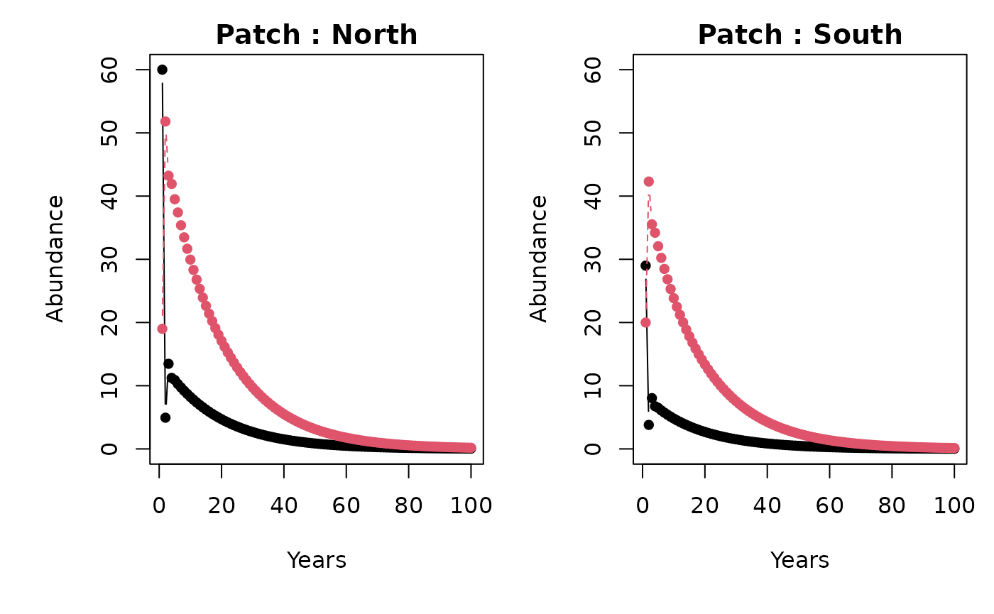
Now we can project populations into future time steps. First, we have to indicate the starting, initial, or current sizes of each stage by patch, or vice versa if grouping by stages. An added step is to comment on the vector which ensures projection calculations are correct. The numbers for n below were retrieved from Table 1 of Wootton and Bell (1992).

n <- c(
  60, 19,  # Northern patch adults then juveniles
  29, 20   # Southern patch adults then juveniles
)
comment(n) <- "patches"  # vector attr for group_by

Now we indicate the number of time steps we would like to project.

n_timesteps <- 100

And, finally we can project stages within patches using the metapopbio::spmm.project function.

head(
  projs <-
    metapopbio::spmm.project(
      n = n,
      A = A,
      n_timesteps = n_timesteps,
      n_stages = n_stages,
      n_patches = n_patches
    )
)
#> [1] "Deterministic spatial matrix model projections for patches structured population vector and movement then demography A projection matrix."
#>       1  2  3  4  5  6  7  8  9 10 11 12 13 14 15 16 17 18 19 20 21 22 23 24 25
#> [1,] 60  4 13 10 10  9  8  8  7  7  6  5  5  4  4  3  3  3  2  2  2  1  1  1  1
#> [2,] 19 51 41 39 36 34 31 29 27 25 23 21 19 17 15 14 12 11 10  8  7  6  5  4  3
#> [3,] 29  3  7  6  6  5  5  4  4  3  3  3  2  2  2  2  1  1  1  1  1  0  0  0  0
#> [4,] 20 42 34 32 29 27 25 23 21 19 17 15 14 12 11 10  9  8  7  6  5  4  3  2  1
#>      26 27 28 29 30 31 32 33 34 35 36 37 38 39 40 41 42 43 44 45 46 47 48 49 50
#> [1,]  0  0  0  0  0  0  0  0  0  0  0  0  0  0  0  0  0  0  0  0  0  0  0  0  0
#> [2,]  2  1  0  0  0  0  0  0  0  0  0  0  0  0  0  0  0  0  0  0  0  0  0  0  0
#> [3,]  0  0  0  0  0  0  0  0  0  0  0  0  0  0  0  0  0  0  0  0  0  0  0  0  0
#> [4,]  0  0  0  0  0  0  0  0  0  0  0  0  0  0  0  0  0  0  0  0  0  0  0  0  0
#>      51 52 53 54 55 56 57 58 59 60 61 62 63 64 65 66 67 68 69 70 71 72 73 74 75
#> [1,]  0  0  0  0  0  0  0  0  0  0  0  0  0  0  0  0  0  0  0  0  0  0  0  0  0
#> [2,]  0  0  0  0  0  0  0  0  0  0  0  0  0  0  0  0  0  0  0  0  0  0  0  0  0
#> [3,]  0  0  0  0  0  0  0  0  0  0  0  0  0  0  0  0  0  0  0  0  0  0  0  0  0
#> [4,]  0  0  0  0  0  0  0  0  0  0  0  0  0  0  0  0  0  0  0  0  0  0  0  0  0
#>      76 77 78 79 80 81 82 83 84 85 86 87 88 89 90 91 92 93 94 95 96 97 98 99
#> [1,]  0  0  0  0  0  0  0  0  0  0  0  0  0  0  0  0  0  0  0  0  0  0  0  0
#> [2,]  0  0  0  0  0  0  0  0  0  0  0  0  0  0  0  0  0  0  0  0  0  0  0  0
#> [3,]  0  0  0  0  0  0  0  0  0  0  0  0  0  0  0  0  0  0  0  0  0  0  0  0
#> [4,]  0  0  0  0  0  0  0  0  0  0  0  0  0  0  0  0  0  0  0  0  0  0  0  0
#>      100
#> [1,]   0
#> [2,]   0
#> [3,]   0
#> [4,]   0

8. Plotting

stage_names <- c("Juv.", "Adults")
patch_names <- c("North", "South")
metapopbio::spmm.plot(
  projections = projs,
  ylabs = "Abundance",
  xlabs = "Years",
  stage_names = stage_names,
  patch_names = patch_names
)

9. Sensitivity and elasticity analyses

metapopbio::spmm.project.matrix.sens(A)
#>            [,1]      [,2]       [,3]      [,4]
#> [1,] 0.10867018 0.3949167 0.06141440 0.3054113
#> [2,] 0.16158007 0.5871958 0.09131616 0.4541115
#> [3,] 0.08404076 0.3054113 0.04749521 0.2361917
#> [4,] 0.09131616 0.3318507 0.05160687 0.2566388
metapopbio::spmm.eig.lambda(A)
#> $eig
#> eigen() decomposition
#> $values
#> [1]  0.94486220  0.85353422 -0.17486220 -0.08353422
#> 
#> $vectors
#>           [,1]       [,2]       [,3]       [,4]
#> [1,] 0.2111729 -0.1455690 -0.6997575  0.5681052
#> [2,] 0.7674202 -0.4778775  0.4706197 -0.1825239
#> [3,] 0.1193433  0.1882302 -0.3954644 -0.7345971
#> [4,] 0.5934892  0.8455839  0.3639567  0.3229684
#> 
#> 
#> $lambda
#> [1] 0.9448622
#> 
#> $v
#> [1] 0.2111729 0.7674202 0.1193433 0.5934892
#> 
#> $eig_t
#> eigen() decomposition
#> $values
#> [1]  0.94486220  0.85353422 -0.17486220 -0.08353422
#> 
#> $vectors
#>            [,1]       [,2]       [,3]       [,4]
#> [1,] -0.4706197 -0.1825239 -0.7674202 -0.4778775
#> [2,] -0.6997575 -0.5681052  0.2111729  0.1455690
#> [3,] -0.3639567  0.3229684 -0.5934892  0.8455839
#> [4,] -0.3954644  0.7345971  0.1193433 -0.1882302
#> 
#> 
#> $w
#> [1] -0.4706197 -0.6997575 -0.3639567 -0.3954644
metapopbio::spmm.demo.sens(BB, A, P, MM)
#>            [,1]       [,2]       [,3]       [,4]
#> [1,] 0.10202024 0.16158007 0.09069071 0.09131616
#> [2,] 0.37075026 0.58719578 0.32957777 0.33185072
#> [3,] 0.05765622 0.09131616 0.05125339 0.05160687
#> [4,] 0.28672202 0.45411152 0.25488102 0.25663882
metapopbio::spmm.demo.elas(BB, A, P, MM)
#>           [,1]       [,2]      [,3]      [,4]
#> [1,] 0.0000000 0.04446238 0.0000000 0.0000000
#> [2,] 0.2825176 0.47852560 0.0000000 0.0000000
#> [3,] 0.0000000 0.00000000 0.0000000 0.0103775
#> [4,] 0.0000000 0.00000000 0.1942234 0.2091436
metapopbio::spmm.move.sens(MM, A, P, BB)
#>           [,1]      [,2]      [,3]      [,4]
#> [1,] 0.2843400 0.2198961 0.4227810 0.2389325
#> [2,] 0.2198961 0.1700581 0.3269603 0.1847800
#> [3,] 0.3323401 0.2570173 0.4941516 0.2792673
#> [4,] 0.2468354 0.1908917 0.3670159 0.2074172
metapopbio::spmm.move.elas(MM, A, P, BB)
#>            [,1]       [,2]     [,3]      [,4]
#> [1,] 0.21968095 0.06283663 0.000000 0.0000000
#> [2,] 0.06283663 0.13138675 0.000000 0.0000000
#> [3,] 0.00000000 0.00000000 0.522988 0.0000000
#> [4,] 0.00000000 0.00000000 0.000000 0.2195211

The black-headed gull

Fewer comments are provided for this example but it should be noted that the grouping (structure of n) is by stages in this example. The life-cycle order remains the same, i.e., movement then demographics (only juveniles assumed to disperse).

1. Patches, stages, and grouping

First, we define the number of patches and stages (age, class, or size). In this example there are two “patches” and five life-stages. We also group or will project patches within stages.

n_patches <- 2
n_stages <- 5
group_by <- "stages"

2. Construct vec-permutation matrix

Next, we construct the vec-permutation matrix.

(P <-
  metapopbio::vec.perm(n_stages = n_stages,
           n_patches = n_patches,
           group_by = group_by))
#>       [,1] [,2] [,3] [,4] [,5] [,6] [,7] [,8] [,9] [,10]
#>  [1,]    1    0    0    0    0    0    0    0    0     0
#>  [2,]    0    0    0    0    0    1    0    0    0     0
#>  [3,]    0    1    0    0    0    0    0    0    0     0
#>  [4,]    0    0    0    0    0    0    1    0    0     0
#>  [5,]    0    0    1    0    0    0    0    0    0     0
#>  [6,]    0    0    0    0    0    0    0    1    0     0
#>  [7,]    0    0    0    1    0    0    0    0    0     0
#>  [8,]    0    0    0    0    0    0    0    0    1     0
#>  [9,]    0    0    0    0    1    0    0    0    0     0
#> [10,]    0    0    0    0    0    0    0    0    0     1

3. Define and structure Demographic parameters

We now specify transition probabilities from one stage to the next. Only adults are assumed to reproduce and differential among adult stages. We will specify demographic parameters and structure the (Leslie-style) matrices for each patch simultaneously.

B1x <- matrix(c(0.000, 0.096, 0.160, 0.224, 0.320,
                0.800, 0.000, 0.000, 0.000, 0.000,
                0.000, 0.820, 0.000, 0.000, 0.000,
                0.000, 0.000, 0.820, 0.000, 0.000,
                0.000, 0.000, 0.000, 0.820, 0.820),
              nrow = n_stages, ncol = n_stages, byrow = TRUE)
B2x <- matrix(c(0.000, 0.100, 0.160, 0.200, 0.200,
                0.800, 0.000, 0.000, 0.000, 0.000,
                0.000, 0.820, 0.000, 0.000, 0.000,
                0.000, 0.000, 0.820, 0.000, 0.000,
                0.000, 0.000, 0.000, 0.820, 0.820),
              nrow = n_stages, ncol = n_stages, byrow = TRUE)

4. Construct block diagonal matrix

(BB <- metapopbio::blk.diag(list(B1x, B2x)))
#>       [,1]  [,2] [,3]  [,4] [,5] [,6] [,7] [,8] [,9] [,10]
#>  [1,]  0.0 0.096 0.16 0.224 0.32  0.0 0.00 0.00 0.00  0.00
#>  [2,]  0.8 0.000 0.00 0.000 0.00  0.0 0.00 0.00 0.00  0.00
#>  [3,]  0.0 0.820 0.00 0.000 0.00  0.0 0.00 0.00 0.00  0.00
#>  [4,]  0.0 0.000 0.82 0.000 0.00  0.0 0.00 0.00 0.00  0.00
#>  [5,]  0.0 0.000 0.00 0.820 0.82  0.0 0.00 0.00 0.00  0.00
#>  [6,]  0.0 0.000 0.00 0.000 0.00  0.0 0.10 0.16 0.20  0.20
#>  [7,]  0.0 0.000 0.00 0.000 0.00  0.8 0.00 0.00 0.00  0.00
#>  [8,]  0.0 0.000 0.00 0.000 0.00  0.0 0.82 0.00 0.00  0.00
#>  [9,]  0.0 0.000 0.00 0.000 0.00  0.0 0.00 0.82 0.00  0.00
#> [10,]  0.0 0.000 0.00 0.000 0.00  0.0 0.00 0.00 0.82  0.82

5. Structure movement parameters

# Juveniles
Mx1 <- matrix(c(0.75, 0.375, 0.25, 0.625),
              nrow = n_patches, ncol = n_patches, byrow = TRUE)
# Adults
Mx5 <- Mx4 <- Mx3 <- Mx2 <-
  diag(nrow = n_patches)

# Block diagonal matrix
(MM <- metapopbio::blk.diag(list(Mx1, Mx2, Mx3, Mx4, Mx5)))
#>       [,1]  [,2] [,3] [,4] [,5] [,6] [,7] [,8] [,9] [,10]
#>  [1,] 0.75 0.375    0    0    0    0    0    0    0     0
#>  [2,] 0.25 0.625    0    0    0    0    0    0    0     0
#>  [3,] 0.00 0.000    1    0    0    0    0    0    0     0
#>  [4,] 0.00 0.000    0    1    0    0    0    0    0     0
#>  [5,] 0.00 0.000    0    0    1    0    0    0    0     0
#>  [6,] 0.00 0.000    0    0    0    1    0    0    0     0
#>  [7,] 0.00 0.000    0    0    0    0    1    0    0     0
#>  [8,] 0.00 0.000    0    0    0    0    0    1    0     0
#>  [9,] 0.00 0.000    0    0    0    0    0    0    1     0
#> [10,] 0.00 0.000    0    0    0    0    0    0    0     1

6. Construct projection matrix

group_by <- "stages"
lh_order <- "move"
(A <-
  metapopbio::spmm.project.matrix(
    P = P,
    BB = BB,
    MM = MM,
    group_by = group_by,
    lh_order = lh_order
  ))
#>       [,1] [,2]  [,3] [,4] [,5] [,6]  [,7] [,8] [,9] [,10]
#>  [1,]  0.0  0.0 0.096 0.00 0.16 0.00 0.224 0.00 0.32  0.00
#>  [2,]  0.0  0.0 0.000 0.10 0.00 0.16 0.000 0.20 0.00  0.20
#>  [3,]  0.6  0.3 0.000 0.00 0.00 0.00 0.000 0.00 0.00  0.00
#>  [4,]  0.2  0.5 0.000 0.00 0.00 0.00 0.000 0.00 0.00  0.00
#>  [5,]  0.0  0.0 0.820 0.00 0.00 0.00 0.000 0.00 0.00  0.00
#>  [6,]  0.0  0.0 0.000 0.82 0.00 0.00 0.000 0.00 0.00  0.00
#>  [7,]  0.0  0.0 0.000 0.00 0.82 0.00 0.000 0.00 0.00  0.00
#>  [8,]  0.0  0.0 0.000 0.00 0.00 0.82 0.000 0.00 0.00  0.00
#>  [9,]  0.0  0.0 0.000 0.00 0.00 0.00 0.820 0.00 0.82  0.00
#> [10,]  0.0  0.0 0.000 0.00 0.00 0.00 0.000 0.82 0.00  0.82

7. Project

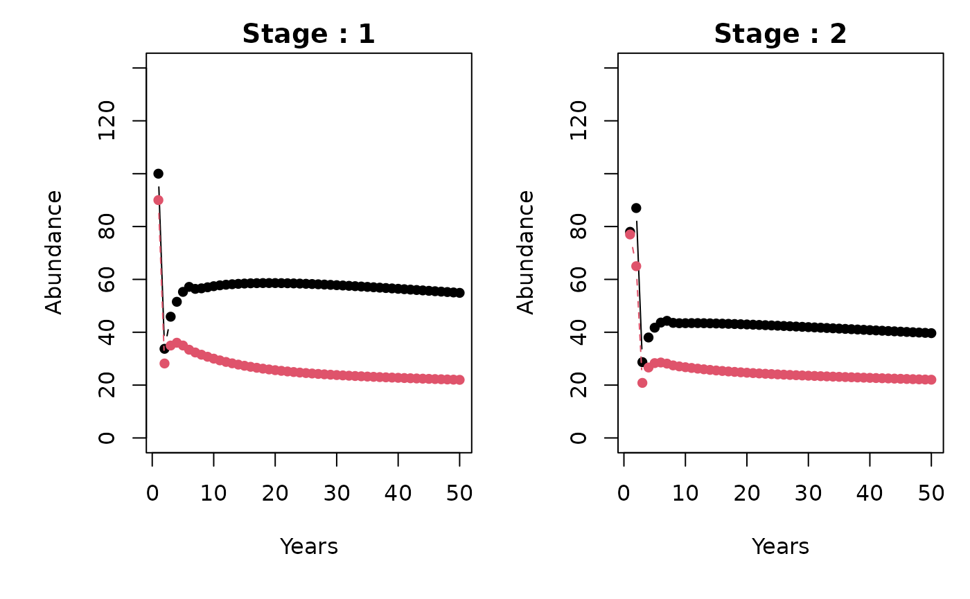
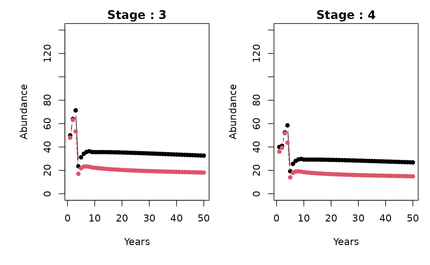
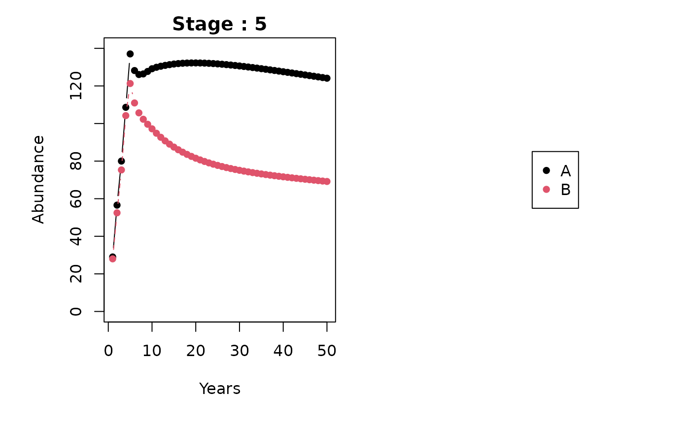
Now we can project populations into future time steps. First, we have to indicate the starting, initial, or current sizes of each patch by stage. I have made these up as they were not avilable in Hunter and Morris (2005) nor Lebreton (1996). An added step is to comment on the vector which ensures projection calculations are correct.

n <- c(
  100, 90,  # stage 1
  78, 77,  # stage 2
  50, 48,  # stage 3
  40, 36,  # stage 4
  29, 28  # stage 5
)
comment(n) <- "stages"  # vector attr for group_by

Now we indicate the number of time steps we would like to project.

n_timesteps <- 50

And, finally we can project stages within patches using the metapopbio::spmm.project function.

head(
  projs <-
    metapopbio::spmm.project(
      n = n,
      A = A,
      n_timesteps = n_timesteps,
      n_stages = n_stages,
      n_patches = n_patches
    )
)
#> [1] "Deterministic spatial matrix model projections for stages structured population vector and movement then demography A projection matrix."
#>        1  2  3  4  5  6  7  8  9 10 11 12 13 14 15 16 17 18 19 20 21 22 23 24
#> [1,] 100 33 45 50 53 55 54 54 53 53 53 53 53 52 52 51 51 50 50 49 49 48 47 47
#> [2,]  90 28 34 35 34 32 31 30 29 28 27 26 25 24 23 23 22 22 21 21 20 19 19 19
#> [3,]  78 87 28 37 40 42 42 41 41 40 40 39 39 39 38 38 37 37 36 36 35 35 34 33
#> [4,]  77 65 20 26 27 27 27 26 25 25 24 24 23 23 22 21 21 21 21 20 20 19 19 18
#> [5,]  50 63 71 22 30 32 34 34 33 33 32 32 31 31 31 31 31 30 30 29 29 28 28 27
#> [6,]  48 63 53 16 21 22 22 22 21 20 20 19 19 18 18 18 17 17 17 17 16 16 15 15
#>      25 26 27 28 29 30 31 32 33 34 35 36 37 38 39 40 41 42 43 44 45 46 47 48 49
#> [1,] 46 45 45 44 44 43 43 42 41 41 40 39 38 37 37 37 36 36 35 35 34 33 33 32 31
#> [2,] 18 18 17 17 16 16 16 15 15 15 14 14 14 13 13 13 12 12 12 12 12 11 11 11 11
#> [3,] 33 33 32 32 31 31 30 30 29 29 29 28 27 27 26 26 26 25 25 24 24 24 23 23 22
#> [4,] 18 18 18 17 17 16 16 16 15 15 15 15 14 14 13 13 13 13 13 13 13 12 12 12 11
#> [5,] 27 27 27 26 26 25 25 24 24 23 23 23 22 22 22 21 21 21 20 20 19 19 19 18 18
#> [6,] 14 14 14 14 13 13 13 13 13 12 12 12 12 11 11 10 10 10 10 10 10 10  9  9  9
#>      50
#> [1,] 31
#> [2,] 10
#> [3,] 21
#> [4,] 11
#> [5,] 18
#> [6,]  9

8. Plotting

stage_names <- as.character(1:5)
patch_names <- c("A", "B")
metapopbio::spmm.plot(
  projections = projs,
  ylabs = "Abundance",
  xlabs = "Years",
  stage_names = stage_names,
  patch_names = patch_names
)

9. Sensitivity and elasticity analyses

metapopbio::spmm.project.matrix.sens(A)
#>                [,1]          [,2]          [,3]          [,4]          [,5]
#>  [1,] 0.09755745+0i 0.03894678+0i 0.07042373+0i 0.03909882+0i 0.05791623+0i
#>  [2,] 0.08124494+0i 0.03243452+0i 0.05864823+0i 0.03256113+0i 0.04823210+0i
#>  [3,] 0.13514559+0i 0.05395267+0i 0.09755745+0i 0.05416329+0i 0.08023091+0i
#>  [4,] 0.08092901+0i 0.03230839+0i 0.05842017+0i 0.03243452+0i 0.04804455+0i
#>  [5,] 0.15291005+0i 0.06104458+0i 0.11038107+0i 0.06128289+0i 0.09077701+0i
#>  [6,] 0.08849839+0i 0.03533023+0i 0.06388427+0i 0.03546815+0i 0.05253820+0i
#>  [7,] 0.16689665+0i 0.06662830+0i 0.12047757+0i 0.06688840+0i 0.09908034+0i
#>  [8,] 0.09175768+0i 0.03663140+0i 0.06623705+0i 0.03677440+0i 0.05447313+0i
#>  [9,] 0.17628954+0i 0.07037812+0i 0.12725801+0i 0.07065286+0i 0.10465655+0i
#> [10,] 0.09175768+0i 0.03663140+0i 0.06623705+0i 0.03677440+0i 0.05447313+0i
#>                [,6]          [,7]          [,8]         [,9]        [,10]
#>  [1,] 0.03215474+0i 0.04763011+0i 0.02644394+0i 0.2205523+0i 0.1224493+0i
#>  [2,] 0.02677817+0i 0.03966592+0i 0.02202227+0i 0.1836739+0i 0.1019746+0i
#>  [3,] 0.04454371+0i 0.06598163+0i 0.03663259+0i 0.3055294+0i 0.1696280+0i
#>  [4,] 0.02667404+0i 0.03951167+0i 0.02193664+0i 0.1829597+0i 0.1015781+0i
#>  [5,] 0.05039884+0i 0.07465471+0i 0.04144783+0i 0.3456903+0i 0.1919251+0i
#>  [6,] 0.02916889+0i 0.04320724+0i 0.02398839+0i 0.2000721+0i 0.1110788+0i
#>  [7,] 0.05500879+0i 0.08148333+0i 0.04523904+0i 0.3773104+0i 0.2094804+0i
#>  [8,] 0.03024314+0i 0.04479851+0i 0.02487186+0i 0.2074405+0i 0.1151697+0i
#>  [9,] 0.05810467+0i 0.08606919+0i 0.04778508+0i 0.3985453+0i 0.2212699+0i
#> [10,] 0.03024314+0i 0.04479851+0i 0.02487186+0i 0.2074405+0i 0.1151697+0i
metapopbio::spmm.eig.lambda(A)
#> $eig
#> eigen() decomposition
#> $values
#>  [1]  9.970859e-01+0.0000000i  8.919222e-01+0.0000000i  2.182849e-01+0.4025870i
#>  [4]  2.182849e-01-0.4025870i -3.024940e-01+0.2461757i -3.024940e-01-0.2461757i
#>  [7]  6.112978e-02+0.2358721i  6.112978e-02-0.2358721i -2.028494e-01+0.0000000i
#> [10]  1.791285e-15+0.0000000i
#> 
#> $vectors
#>                 [,1]           [,2]                     [,3]
#>  [1,] -0.32790653+0i -0.18212972+0i  0.116056424-0.07487059i
#>  [2,] -0.13090649+0i  0.22690373+0i  0.006076633+0.01670070i
#>  [3,] -0.23670566+0i -0.04619989+0i -0.002241819-0.17870968i
#>  [4,] -0.13141752+0i  0.08635946+0i  0.014606045-0.05728283i
#>  [5,] -0.19466592+0i -0.04247446+0i -0.283215006-0.14899452i
#>  [6,] -0.10807732+0i  0.07939566+0i -0.077701404-0.07188011i
#>  [7,] -0.16009259+0i -0.03904943+0i -0.476243342+0.31863815i
#>  [8,] -0.08888242+0i  0.07299341+0i -0.179460166+0.06096001i
#>  [9,] -0.74131229+0i -0.44521053+0i  0.649010676+0.00000000i
#> [10,] -0.41157200+0i  0.83221273+0i  0.207333032+0.05564490i
#>                           [,4]                      [,5]
#>  [1,]  0.116056424+0.07487059i  0.05022988+0.0927743125i
#>  [2,]  0.006076633-0.01670070i -0.00445866-0.0004872395i
#>  [3,] -0.002241819+0.17870968i  0.03257850-0.1570225501i
#>  [4,]  0.014606045+0.05728283i  0.01409087-0.0490667965i
#>  [5,] -0.283215006+0.14899452i -0.26151751+0.2128281605i
#>  [6,] -0.077701404+0.07188011i -0.08809695+0.0613150917i
#>  [7,] -0.476243342-0.31863815i  0.70892098+0.0000000000i
#>  [8,] -0.179460166-0.06096001i  0.22503737+0.0169271029i
#>  [9,]  0.649010676+0.00000000i -0.49411266-0.1083645061i
#> [10,]  0.207333032-0.05564490i -0.15426192-0.0461969101i
#>                            [,6]                      [,7]
#>  [1,]  0.05022988-0.0927743125i  0.014698188+0.010441279i
#>  [2,] -0.00445866+0.0004872395i -0.031370628-0.018391363i
#>  [3,]  0.03257850+0.1570225501i  0.002359263+0.003122440i
#>  [4,]  0.01409087+0.0490667965i -0.041358939+0.043317596i
#>  [5,] -0.26151751-0.2128281605i  0.012163687-0.005049481i
#>  [6,] -0.08809695-0.0613150917i  0.106195671+0.171304886i
#>  [7,]  0.70892098+0.0000000000i -0.006180033-0.043888220i
#>  [8,]  0.22503737-0.0169271029i  0.647709984-0.201321292i
#>  [9,] -0.49411266+0.1083645061i -0.007352067+0.045138406i
#> [10,] -0.15426192+0.0461969101i -0.699885399+0.000000000i
#>                            [,8]            [,9]            [,10]
#>  [1,]  0.014698188-0.010441279i  0.010988584+0i -5.224894e-16+0i
#>  [2,] -0.031370628+0.018391363i -0.023369498+0i -3.630818e-17+0i
#>  [3,]  0.002359263-0.003122440i  0.002059156+0i  1.699276e-16+0i
#>  [4,] -0.041358939-0.043317596i  0.046768853+0i  1.250305e-16+0i
#>  [5,]  0.012163687+0.005049481i -0.008323952+0i -2.213028e-17+0i
#>  [6,]  0.106195671-0.171304886i -0.189058814+0i -1.216778e-15+0i
#>  [7,] -0.006180033+0.043888220i  0.033648815+0i  1.660406e-15+0i
#>  [8,]  0.647709984+0.201321292i  0.764252980+0i -7.071068e-01+0i
#>  [9,] -0.007352067-0.045138406i -0.026975652+0i -1.566664e-15+0i
#> [10,] -0.699885399+0.000000000i -0.612687917+0i  7.071068e-01+0i
#> 
#> 
#> $lambda
#> [1] 0.9970859
#> 
#> $v
#>  [1] -0.32790653+0i -0.13090649+0i -0.23670566+0i -0.13141752+0i -0.19466592+0i
#>  [6] -0.10807732+0i -0.16009259+0i -0.08888242+0i -0.74131229+0i -0.41157200+0i
#> 
#> $eig_t
#> eigen() decomposition
#> $values
#>  [1]  9.970859e-01+0.0000000i  8.919222e-01+0.0000000i  2.182849e-01+0.4025870i
#>  [4]  2.182849e-01-0.4025870i -3.024940e-01+0.2461757i -3.024940e-01-0.2461757i
#>  [7]  6.112978e-02+0.2358721i  6.112978e-02-0.2358721i -2.028494e-01+0.0000000i
#> [10]  1.718711e-15+0.0000000i
#> 
#> $vectors
#>               [,1]           [,2]                    [,3]
#>  [1,] 0.2536597+0i  0.05633004+0i  0.62139103+0.00000000i
#>  [2,] 0.2112455+0i -0.15794294+0i  0.29776448+0.07991527i
#>  [3,] 0.3513929+0i  0.22206487+0i  0.25523002+0.40674126i
#>  [4,] 0.2104240+0i -0.41498457+0i -0.08748875+0.03059607i
#>  [5,] 0.3975824+0i  0.23494746+0i -0.20449932+0.23358264i
#>  [6,] 0.2301052+0i -0.43212154+0i -0.07462378-0.04455451i
#>  [7,] 0.4339490+0i  0.24456348+0i -0.29036465-0.03822100i
#>  [8,] 0.2385797+0i -0.43920480+0i -0.05609084-0.06409096i
#>  [9,] 0.4583715+0i  0.25062643+0i -0.22827625-0.15273184i
#> [10,] 0.2385797+0i -0.43920480+0i -0.05609084-0.06409096i
#>                          [,4]                      [,5]
#>  [1,]  0.62139103+0.00000000i -0.731336362+0.000000000i
#>  [2,]  0.29776448-0.07991527i -0.348229238-0.026193482i
#>  [3,]  0.25523002-0.40674126i  0.367730607-0.310242367i
#>  [4,] -0.08748875-0.03059607i  0.002932555+0.030541037i
#>  [5,] -0.20449932-0.23358264i  0.043105002+0.224844860i
#>  [6,] -0.07462378+0.04455451i  0.032216321-0.007191719i
#>  [7,] -0.29036465+0.03822100i  0.059296927-0.070003443i
#>  [8,] -0.05609084+0.06409096i  0.058221780+0.017435711i
#>  [9,] -0.22827625+0.15273184i  0.198921369+0.043625711i
#> [10,] -0.05609084+0.06409096i  0.058221780+0.017435711i
#>                            [,6]                     [,7]
#>  [1,] -0.731336362+0.000000000i  0.005488647-0.03369784i
#>  [2,] -0.348229238+0.026193482i  0.783743606+0.00000000i
#>  [3,]  0.367730607+0.310242367i -0.022666936-0.15564715i
#>  [4,]  0.002932555-0.030541037i  0.109420309+0.46311484i
#>  [5,]  0.043105002-0.224844860i  0.042439378-0.01417827i
#>  [6,]  0.032216321+0.007191719i -0.220635858+0.06599916i
#>  [7,]  0.059296927+0.070003443i  0.006171201+0.01772586i
#>  [8,]  0.058221780-0.017435711i -0.188358244-0.05854553i
#>  [9,]  0.198921369-0.043625711i -0.006138109+0.01230184i
#> [10,]  0.058221780-0.017435711i -0.188358244-0.05854553i
#>                           [,8]            [,9]            [,10]
#>  [1,]  0.005488647+0.03369784i -0.025230343+0i -5.295556e-15+0i
#>  [2,]  0.783743606+0.00000000i -0.859571041+0i -9.481194e-01+0i
#>  [3,] -0.022666936+0.15564715i -0.134640449+0i  1.193352e-15+0i
#>  [4,]  0.109420309-0.46311484i  0.429511140+0i -4.231046e-15+0i
#>  [5,]  0.042439378+0.01417827i  0.036260783+0i  7.478823e-16+0i
#>  [6,] -0.220635858-0.06599916i -0.001425556+0i  1.156243e-01+0i
#>  [7,]  0.006171201-0.01772586i -0.004047100+0i  1.177518e-15+0i
#>  [8,] -0.188358244+0.05854553i  0.168073829+0i  1.849989e-01+0i
#>  [9,] -0.006138109-0.01230184i  0.007893352+0i  1.767433e-15+0i
#> [10,] -0.188358244+0.05854553i  0.168073829+0i  2.312486e-01+0i
#> 
#> 
#> $w
#>  [1] 0.2536597+0i 0.2112455+0i 0.3513929+0i 0.2104240+0i 0.3975824+0i
#>  [6] 0.2301052+0i 0.4339490+0i 0.2385797+0i 0.4583715+0i 0.2385797+0i
metapopbio::spmm.demo.sens(BB, A, P, MM)
#>                [,1]          [,2]          [,3]          [,4]          [,5]
#>  [1,] 0.10635498+0i 0.08124494+0i 0.13514559+0i 0.08092901+0i 0.15291005+0i
#>  [2,] 0.04245892+0i 0.03243452+0i 0.05395267+0i 0.03230839+0i 0.06104458+0i
#>  [3,] 0.07677440+0i 0.05864823+0i 0.09755745+0i 0.05842017+0i 0.11038107+0i
#>  [4,] 0.04262467+0i 0.03256113+0i 0.05416329+0i 0.03243452+0i 0.06128289+0i
#>  [5,] 0.06313900+0i 0.04823210+0i 0.08023091+0i 0.04804455+0i 0.09077701+0i
#>  [6,] 0.03505438+0i 0.02677817+0i 0.04454371+0i 0.02667404+0i 0.05039884+0i
#>  [7,] 0.05192530+0i 0.03966592+0i 0.06598163+0i 0.03951167+0i 0.07465471+0i
#>  [8,] 0.02882861+0i 0.02202227+0i 0.03663259+0i 0.02193664+0i 0.04144783+0i
#>  [9,] 0.24044125+0i 0.18367391+0i 0.30552940+0i 0.18295967+0i 0.34569027+0i
#> [10,] 0.13349150+0i 0.10197462+0i 0.16962803+0i 0.10157808+0i 0.19192510+0i
#>                [,6]          [,7]          [,8]          [,9]         [,10]
#>  [1,] 0.07970085+0i 0.16689665+0i 0.09175768+0i 0.17628954+0i 0.09175768+0i
#>  [2,] 0.03181809+0i 0.06662830+0i 0.03663140+0i 0.07037812+0i 0.03663140+0i
#>  [3,] 0.05753360+0i 0.12047757+0i 0.06623705+0i 0.12725801+0i 0.06623705+0i
#>  [4,] 0.03194230+0i 0.06688840+0i 0.03677440+0i 0.07065286+0i 0.03677440+0i
#>  [5,] 0.04731544+0i 0.09908034+0i 0.05447313+0i 0.10465655+0i 0.05447313+0i
#>  [6,] 0.02626924+0i 0.05500879+0i 0.03024314+0i 0.05810467+0i 0.03024314+0i
#>  [7,] 0.03891205+0i 0.08148333+0i 0.04479851+0i 0.08606919+0i 0.04479851+0i
#>  [8,] 0.02160373+0i 0.04523904+0i 0.02487186+0i 0.04778508+0i 0.02487186+0i
#>  [9,] 0.18018313+0i 0.37731038+0i 0.20744051+0i 0.39854528+0i 0.20744051+0i
#> [10,] 0.10003656+0i 0.20948039+0i 0.11516969+0i 0.22126988+0i 0.11516969+0i
metapopbio::spmm.demo.elas(BB, A, P, MM)
#>                [,1]          [,2]          [,3]          [,4]          [,5]
#>  [1,] 0.00000000+0i 0.00782231+0i 0.02168649+0i 0.01818108+0i 0.04907422+0i
#>  [2,] 0.03406641+0i 0.00000000+0i 0.00000000+0i 0.00000000+0i 0.00000000+0i
#>  [3,] 0.00000000+0i 0.04823210+0i 0.00000000+0i 0.00000000+0i 0.00000000+0i
#>  [4,] 0.00000000+0i 0.00000000+0i 0.04454371+0i 0.00000000+0i 0.00000000+0i
#>  [5,] 0.00000000+0i 0.00000000+0i 0.00000000+0i 0.03951167+0i 0.07465471+0i
#>  [6,] 0.00000000+0i 0.00000000+0i 0.00000000+0i 0.00000000+0i 0.00000000+0i
#>  [7,] 0.00000000+0i 0.00000000+0i 0.00000000+0i 0.00000000+0i 0.00000000+0i
#>  [8,] 0.00000000+0i 0.00000000+0i 0.00000000+0i 0.00000000+0i 0.00000000+0i
#>  [9,] 0.00000000+0i 0.00000000+0i 0.00000000+0i 0.00000000+0i 0.00000000+0i
#> [10,] 0.00000000+0i 0.00000000+0i 0.00000000+0i 0.00000000+0i 0.00000000+0i
#>                [,6]           [,7]           [,8]         [,9]          [,10]
#>  [1,] 0.00000000+0i 0.000000000+0i 0.000000000+0i 0.0000000+0i 0.000000000+0i
#>  [2,] 0.00000000+0i 0.000000000+0i 0.000000000+0i 0.0000000+0i 0.000000000+0i
#>  [3,] 0.00000000+0i 0.000000000+0i 0.000000000+0i 0.0000000+0i 0.000000000+0i
#>  [4,] 0.00000000+0i 0.000000000+0i 0.000000000+0i 0.0000000+0i 0.000000000+0i
#>  [5,] 0.00000000+0i 0.000000000+0i 0.000000000+0i 0.0000000+0i 0.000000000+0i
#>  [6,] 0.00000000+0i 0.005516956+0i 0.004853045+0i 0.0116549+0i 0.006066307+0i
#>  [7,] 0.03122062+0i 0.000000000+0i 0.000000000+0i 0.0000000+0i 0.000000000+0i
#>  [8,] 0.00000000+0i 0.037204434+0i 0.000000000+0i 0.0000000+0i 0.000000000+0i
#>  [9,] 0.00000000+0i 0.000000000+0i 0.170598367+0i 0.0000000+0i 0.000000000+0i
#> [10,] 0.00000000+0i 0.000000000+0i 0.000000000+0i 0.1819716+0i 0.094715159+0i
metapopbio::spmm.move.sens(MM, A, P, BB)
#>                [,1]          [,2]          [,3]          [,4]          [,5]
#>  [1,] 0.03115742+0i 0.02826418+0i 0.02594761+0i 0.05330264+0i 0.04316214+0i
#>  [2,] 0.03810409+0i 0.03456579+0i 0.03173273+0i 0.06518667+0i 0.05278530+0i
#>  [3,] 0.06711297+0i 0.06088095+0i 0.05589106+0i 0.11481368+0i 0.09297109+0i
#>  [4,] 0.02489951+0i 0.02258737+0i 0.02073608+0i 0.04259689+0i 0.03449310+0i
#>  [5,] 0.04767022+0i 0.04324363+0i 0.03969932+0i 0.08155195+0i 0.06603719+0i
#>  [6,] 0.18599764+0i 0.16872613+0i 0.15489711+0i 0.31819592+0i 0.25766110+0i
#>  [7,] 0.06934418+0i 0.06290497+0i 0.05774919+0i 0.11863073+0i 0.09606196+0i
#>  [8,] 0.10683935+0i 0.09691838+0i 0.08897482+0i 0.18277568+0i 0.14800373+0i
#>  [9,] 0.07870970+0i 0.07140081+0i 0.06554871+0i 0.13465281+0i 0.10903594+0i
#> [10,] 0.10683935+0i 0.09691838+0i 0.08897482+0i 0.18277568+0i 0.14800373+0i
#>                [,6]          [,7]          [,8]          [,9]         [,10]
#>  [1,] 0.02930512+0i 0.02584671+0i 0.05630249+0i 0.04883567+0i 0.02930512+0i
#>  [2,] 0.03583881+0i 0.03160934+0i 0.06885535+0i 0.05972376+0i 0.03583881+0i
#>  [3,] 0.06312312+0i 0.05567372+0i 0.12127536+0i 0.10519184+0i 0.06312312+0i
#>  [4,] 0.02341924+0i 0.02065544+0i 0.04499423+0i 0.03902711+0i 0.02341924+0i
#>  [5,] 0.04483624+0i 0.03954495+0i 0.08614167+0i 0.07471758+0i 0.04483624+0i
#>  [6,] 0.17494012+0i 0.15429477+0i 0.33610388+0i 0.29152984+0i 0.17494012+0i
#>  [7,] 0.06522169+0i 0.05752463+0i 0.12530723+0i 0.10868900+0i 0.06522169+0i
#>  [8,] 0.10048777+0i 0.08862883+0i 0.19306223+0i 0.16745835+0i 0.10048777+0i
#>  [9,] 0.07403042+0i 0.06529381+0i 0.14223102+0i 0.12336837+0i 0.07403042+0i
#> [10,] 0.10048777+0i 0.08862883+0i 0.19306223+0i 0.16745835+0i 0.10048777+0i
metapopbio::spmm.move.elas(MM, A, P, BB)
#>                 [,1]          [,2]          [,3]          [,4]         [,5]
#>  [1,] 0.023436364+0i 0.01063005+0i 0.00000000+0i 0.00000000+0i 0.0000000+0i
#>  [2,] 0.009553864+0i 0.02166676+0i 0.00000000+0i 0.00000000+0i 0.0000000+0i
#>  [3,] 0.000000000+0i 0.00000000+0i 0.05605441+0i 0.00000000+0i 0.0000000+0i
#>  [4,] 0.000000000+0i 0.00000000+0i 0.00000000+0i 0.04272139+0i 0.0000000+0i
#>  [5,] 0.000000000+0i 0.00000000+0i 0.00000000+0i 0.00000000+0i 0.0662302+0i
#>  [6,] 0.000000000+0i 0.00000000+0i 0.00000000+0i 0.00000000+0i 0.0000000+0i
#>  [7,] 0.000000000+0i 0.00000000+0i 0.00000000+0i 0.00000000+0i 0.0000000+0i
#>  [8,] 0.000000000+0i 0.00000000+0i 0.00000000+0i 0.00000000+0i 0.0000000+0i
#>  [9,] 0.000000000+0i 0.00000000+0i 0.00000000+0i 0.00000000+0i 0.0000000+0i
#> [10,] 0.000000000+0i 0.00000000+0i 0.00000000+0i 0.00000000+0i 0.0000000+0i
#>               [,6]          [,7]         [,8]         [,9]        [,10]
#>  [1,] 0.0000000+0i 0.00000000+0i 0.0000000+0i 0.0000000+0i 0.0000000+0i
#>  [2,] 0.0000000+0i 0.00000000+0i 0.0000000+0i 0.0000000+0i 0.0000000+0i
#>  [3,] 0.0000000+0i 0.00000000+0i 0.0000000+0i 0.0000000+0i 0.0000000+0i
#>  [4,] 0.0000000+0i 0.00000000+0i 0.0000000+0i 0.0000000+0i 0.0000000+0i
#>  [5,] 0.0000000+0i 0.00000000+0i 0.0000000+0i 0.0000000+0i 0.0000000+0i
#>  [6,] 0.1754514+0i 0.00000000+0i 0.0000000+0i 0.0000000+0i 0.0000000+0i
#>  [7,] 0.0000000+0i 0.05769275+0i 0.0000000+0i 0.0000000+0i 0.0000000+0i
#>  [8,] 0.0000000+0i 0.00000000+0i 0.1936265+0i 0.0000000+0i 0.0000000+0i
#>  [9,] 0.0000000+0i 0.00000000+0i 0.0000000+0i 0.1237289+0i 0.0000000+0i
#> [10,] 0.0000000+0i 0.00000000+0i 0.0000000+0i 0.0000000+0i 0.1007815+0i

References

Caswell, H. (2001). Matrix Population Models: Construction, analysis, and interpretation (2nd ed.). Sinauer Associates.

Gotelli, N. J. (1991). Metapopulation models: the rescue effect, the propagate rain, and the core-satellite hypothesis. The American Naturalist 138(3):768–776.

Gotelli, N. J. (2008). A Primer of Ecology (4th ed.). Sinauer Associates.

Hunter, C. M. and Caswell, H. (2005). The use of vec-permutation matrix in spatial matrix population models. Ecological Modelling 188:15–21.

Lebreton, J. D. (1996). Demographic models for subdivided populations: the renewal equation approach. Theoretical Population Biology 49:291–313.

Leslie, P. H. (1945). On the use of matrices in certain population mathematics. Biometrika 33:183–212.

Morris, W. F., and Doak, D. F. (2003). Quantitative Conservation Biology: Theory and practice of population viability analysis. Sinauer Associates.

Roth, G. and Caswell, H. (2016). Hyperstate matrix models: extending demographic state spaces to higher dimensions. Methods in Ecology and Evolution 7:1438–1450.

Wootton, J.T., and Bell, D.A. (1992). A metapopulation model of the peregrine falcon in California: viability and management strategies. Ecological Applications 2:307-–321.

Caleb A. Aldridge

2024-12-06

About

Examples

The peregrine falcon

1. Patches, stages, and grouping

2. Construct vec-permutation matrix

3. Demographic parameters for each patch

4a. Structure demographic parameters

4b. Construct block diagonal matrix

5. Structure movement parameters

6. Construct projection matrix

7. Project

8. Plotting

9. Sensitivity and elasticity analyses

The black-headed gull

1. Patches, stages, and grouping

2. Construct vec-permutation matrix

3. Define and structure Demographic parameters

4. Construct block diagonal matrix

5. Structure movement parameters

6. Construct projection matrix

7. Project

8. Plotting

9. Sensitivity and elasticity analyses

References